Package {FINN}

Type:	Package
Title:	Forest Informed Neural Networks
Version:	0.1.0
Maintainer:	Yannek Käber <y.kaeber@posteo.de>
Description:	A hybrid dynamic forest (gap) model (FINN) that can be configured as a fully mechanistic, process-based model, like classic forest gap models, or with its demographic processes (growth, mortality, regeneration) replaced by deep neural networks (DNNs), or any combination of the two. Provides functions to define a model and its mechanistic or empirical components, calibrate it to forest inventory data, and interpret the calibrated processes. FINN is implemented with the 'torch' package, which supplies GPU support and the automatic differentiation used to calibrate the model by stochastic gradient descent; no knowledge of 'torch' is required. The hybrid modeling approach is described in Pichler and Käber (2026) <doi:10.1111/2041-210x.70347>.
License:	GPL (≥ 3)
Encoding:	UTF-8
URL:	https://github.com/FINNverse/FINN, https://finnverse.github.io/FINN/
BugReports:	https://github.com/FINNverse/FINN/issues
Depends:	R (≥ 4.1.0)
LinkingTo:	Rcpp
Imports:	abind, cli, stats, utils, data.table, coro, Rcpp, torch, ggplot2, glue
Suggests:	testthat (≥ 3.0.0), knitr, rmarkdown
RoxygenNote:	7.3.3
VignetteBuilder:	knitr
Config/testthat/edition:	3
NeedsCompilation:	yes
Packaged:	2026-08-05 08:00:45 UTC; yannekkaber
Author:	Yannek Käber [aut, cre], Maximilian Pichler [aut]
Repository:	CRAN
Date/Publication:	2026-08-09 08:00:08 UTC

FINN: Forest Informed Neural Networks

Description

FINN is a differentiable forest gap model. A forest is represented as cohorts of same-species, same-size trees that are updated each timestep by four demographic processes — competition, growth, mortality and regeneration. Each process can be a mechanistic function, a neural network, or a mixture of the two, and the whole model is calibrated end-to-end by gradient descent through the simulation (implemented in torch).

Getting started

• finn() assembles a model from one process per component, each built with createProcess() (mechanistic) or createHybrid() (neural network).

• simulateForest() runs a model forward from known parameters.

• fit() calibrates a model to data; predict.finn_class() scores it.

• makeObsData(), resolveSiteIDs() and makeInitCohorts() turn a raw tree list into FINN's input tables.

• ALE(), summary.finn_class(), feature_importance() and conditionalEffects() interpret a fitted model.

The vignettes give a guided tour: browseVignettes("FINN").

Author(s)

Maintainer: Yannek K<c3><a4>ber y.kaeber@posteo.de (ORCID)

Authors:

• Maximilian Pichler maximilian.pichler@biologie.uni-regensburg.de (ORCID)

See Also

Useful links:

• https://github.com/FINNverse/FINN

• https://finnverse.github.io/FINN/

• Report bugs at https://github.com/FINNverse/FINN/issues

Accumulated local effect plots

Description

Calculates accumulated local effects (ALE) for the three processes

Usage

ALE(
  model,
  env = NULL,
  init_cohort = NULL,
  env_autoscale = TRUE,
  sim_seed = 42L,
  plot = TRUE,
  process = NULL,
  scale = FALSE,
  ...
)

Arguments

Value

A list with one table per process (e.g. ⁠$growth⁠, ⁠$mortality⁠, ⁠$regeneration⁠). Each table gives the accumulated local effect (ale) of every driver (var) across its observed range (x), per species. When plot = TRUE the effects are also drawn.

Calculate the Basal Area of a Stand

Description

This function calculates the basal area of a stand based on the diameter at breast height (dbh), the number of trees, and the patch size in hectares.

Usage

BA_stand(dbh, trees, patch_size_ha)

Arguments

Details

The basal area of a stand is the cross-sectional area of all trees in a stand per unit area. This function calculates the basal area per ha using the formula:

BA = \left( \frac{\pi \left( \frac{\text{dbh}}{100} \right)^2}{4} \right) \times \text{trees} \div \text{patch\_size\_ha}

The formula takes into account the diameter at breast height (dbh) in centimeters, the number of trees, and the size of the patch in hectares to calculate the basal area in square meters per hectare.

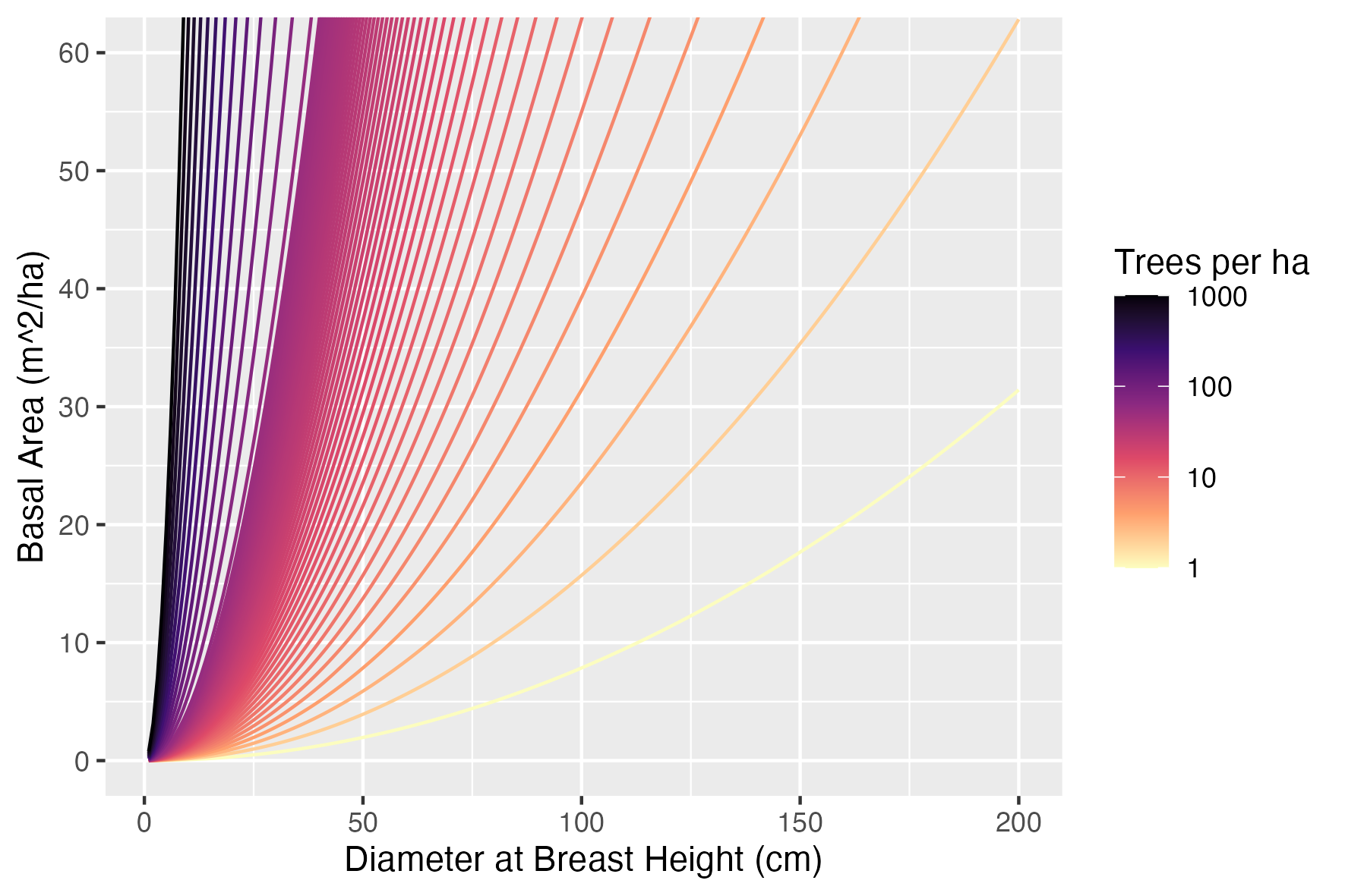
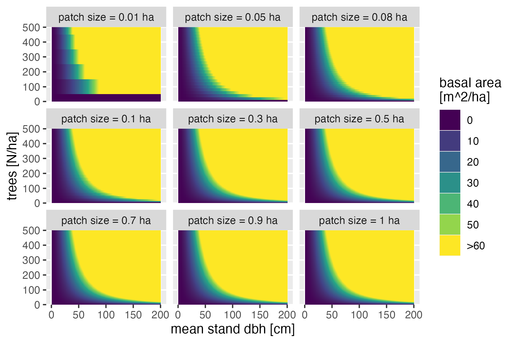
This plot illustrates the basal area for different combinations of dbh and number of trees.

Sensitivity of basal area for different combinations of dbh, number of trees to patch size.

Value

A numeric value representing the basal area of the stand in square meters per hectare.

Examples

# BA_stand operates on torch tensors, so this runs only where the torch
# backend (libtorch) is available.
dbh_vec <- seq(1, 200, 1)
trees_vec <- c(0:500, 10^(seq(2, 4, length.out = 20)))

# Generate test data for a patch size of 0.1
patch_size <- 0.1
cohort_df1 <- expand.grid(
  trees_ha = trees_vec,
  patch_size_ha = patch_size,
  dbh = dbh_vec
)

cohort_df1 <- data.frame(
  patchID = 1,
  cohortID = 1,
  species = 1,
  cohort_df1
)

cohort_df1$siteID <- 1:nrow(cohort_df1)
cohort_df1$trees <- round(cohort_df1$trees_ha * patch_size)

cohort <- CohortMat$new(obs_df = cohort_df1)

cohort_df1$basal_area <- torch::as_array(
  BA_stand(cohort$dbh, cohort$trees, patch_size_ha = patch_size))

# View the first few rows of the resulting data frame
head(cohort_df1)

Calculate the basal area of a tree given the diameter at breast height (dbh)

Description

This function calculates the basal area of a tree given the diameter at breast height (dbh).

Usage

BA_stem(dbh)

Arguments

Value

torch.Tensor The basal area of the tree.

Examples

dbh = torch::torch_tensor(50)
basal_area = BA_stem(dbh)
print(basal_area)

Cohort Matrix Class

Description

Initialize the CohortMat class

Usage

CohortMat(
  obs_df = NULL,
  dbh = NULL,
  trees = NULL,
  species = NULL,
  dims = c(50, 30, 10),
  sp = 10,
  device = "cpu"
)

Arguments

Details

An R6 class for managing cohorts of trees in forest models. This class allows for the initialization, transformation, and manipulation of cohorts represented by arrays of dbh, trees, and species.

Value

data.table object

Fields

dbh

A tensor representing the diameter at breast height for each cohort.

trees

A tensor representing the number of trees in each cohort.

species

A tensor representing the species of each cohort.

dims

A vector representing the dimensions of the arrays (sites, patches, cohorts).

sp

An integer representing the number of species.

device

A character string specifying the device to use ('cpu' or 'cuda').

dbh_r

A numeric array representing the diameter at breast height in R array format.

trees_r

A numeric array representing the number of trees in R array format.

species_r

An integer array representing the species in R array format.

device_r

A character string specifying the device in R format ('cpu' or 'cuda').

obsDF2arrays

Transforms data.table into array

Set Seed for Reproducibility in R and Torch

Description

This function sets the seed for both R's random number generator and Torch's random number generator, ensuring reproducibility across operations that involve both R and Torch.

Usage

FINN.seed(seed)

Arguments

Details

The function calls set.seed() to set the seed for R's random number generator and torch::torch_manual_seed() to set the seed for Torch's random number generator. This is useful for ensuring reproducibility in scripts that rely on both R and Torch for random operations.

Value

This function does not return a value. It sets the seed internally for both R and Torch.

Examples

FINN.seed(123)
# Now both R and Torch are seeded with 123, ensuring reproducible results

Aggregate function

Description

Aggregate function

Usage

aggregate_results_old(
  labels,
  samples,
  Results,
  drop_rows = TRUE,
  sp_max = NULL
)

Arguments

Value

A list of torch tensors, one per element of samples, each holding the per-species aggregated result.

Apply stored z-standardization to environmental predictors

Description

Re-applies the constants learned by compute_env_scaling() to env. The transformation uses the stored mean/sd only and never recomputes them from env, so calibration and prediction use an identical transformation (the usual pitfall of scale() inside a model formula is avoided).

Usage

apply_env_scaling(env, scaling)

Arguments

Value

env with the scaled predictor columns, as a data.table.

See Also

compute_env_scaling, fit

Examples

# reproduce the standardization a model fit with env_autoscale = TRUE used:
env <- data.frame(siteID = 1:3, year = 1L, temp = c(4, 6, 8), prec = c(700, 850, 1000))
scaling <- compute_env_scaling(env)
apply_env_scaling(env, scaling)

Transform Arrays to Observation Data Table

Description

This function transforms arrays of species, dbh, and trees back into an observation data table.

Usage

array2obsDF(obs_array)

Arguments

Value

A data.frame with columns siteID, patchID, cohortID, species, dbh, and trees.

Examples

obs_array <- list(
  species = array(c("A", "B"), dim = c(2, 2, 2)),
  dbh = array(c(10, 20, 30, 40), dim = c(2, 2, 2)),
  trees = array(c(100, 200, 150, 250), dim = c(2, 2, 2)))
result <- array2obsDF(obs_array)

Average conditional effects of a FINN model

Description

Summarises the conditional effects into a per process x species x variable average marginal effect: the mean local derivative (mean_effect, an approximate linear effect). Derived cheaply from the cached conditional effects.

Usage

averageConditionalEffects(
  model,
  env = NULL,
  init_cohort = NULL,
  env_autoscale = TRUE,
  sim_seed = 42L,
  env_only = TRUE
)

Arguments

Value

a named list (one entry per process) of data.frames with columns ⁠species, variable, mean_effect⁠.

Draw binomial counts from per-trial Bernoulli probabilities

Description

Draw binomial counts from per-trial Bernoulli probabilities

Usage

binomial_from_bernoulli(n, p)

Arguments

Value

torch.Tensor The number of successes per element.

Sample from binomial with gradient

Description

Sample from binomial with gradient

Usage

binomial_from_gamma(n, p, sample_size = 1)

Arguments

Value

A torch tensor of binomial samples drawn via the gamma-Poisson relationship.

Convert a climate data frame to a FINN environment array

Description

Reshapes a long-format climate table into the site x year x variable array FINN uses internally, auto-detecting the time resolution from the columns.

Usage

climateDF2array(climate_dt, env_vars)

Arguments

Value

A numeric array of environmental values indexed by site, time and variable.

Compute the fraction of available light (light) for each cohort based on the given parameters

Description

This function calculates the fraction of available light for each cohort of trees based on their diameter at breast height (dbh), species, number of trees, and global parameters.

Usage

competition(
  dbh,
  species,
  trees,
  parComp,
  h = NULL,
  patch_size_ha,
  ba = NULL,
  cohortHeights = NULL,
  n_quantiles = 10,
  continuous = FALSE
)

Arguments

Value

torch.Tensor Fraction of available light (light) for each cohort.

Learn z-standardization for environmental predictors

Description

Computes the centering and scaling constants (mean and standard deviation) of every numeric environmental predictor in env (all columns except the keys siteID and year), so they can be re-applied unchanged to new data at prediction time. A predictor with (near-)zero standard deviation is given scale = 1 (centred only) to avoid division by zero, mirroring recipes::step_normalize.

Usage

compute_env_scaling(env)

Arguments

Value

A data.frame with columns variable, center, scale; or NULL if there are no numeric predictors. This is the object stored on a fitted model as model$env_scaling when it is fit with env_autoscale = TRUE.

See Also

apply_env_scaling

Conditional effects of a FINN model

Description

Computes (and caches on the model) the conditional effects — the local derivatives of each demographic process (growth, mortality, regeneration) with respect to its inputs, per process and per species. This is the shared primitive behind ALE(), averageConditionalEffects() and the analytical variable importance in summary.finn_class().

Usage

conditionalEffects(
  model,
  env = NULL,
  init_cohort = NULL,
  env_autoscale = TRUE,
  sim_seed = 42L
)

Arguments

Value

an object of class FINNconditionalEffects (also cached on model$conditional_effects).

Define a hybrid (deep-neural-network) demographic process for FINN

Description

Configures a process (growth, mortality, or regeneration) in which the entire process equation – not just its environmental-response function – is replaced by a deep neural network (DNN), for use as growth_process, mortality_process, or regeneration_process in finn(). This is the second ("Level 2") level of hybridization described by Pichler & Käber (2026); to replace only the environmental-response function while keeping the rest of the process mechanistic ("Level 1"), use createProcess() instead. competition_process must always be created with createProcess(), as the competition (light availability) process does not support full replacement by a DNN.

Usage

createHybrid(
  formula = NULL,
  optimize = TRUE,
  dispersion_parameter = 1,
  NN = NULL,
  dropout = 0.3,
  encoder_layers = 1L,
  hidden = c(50L, 50L),
  sample_regeneration = TRUE,
  transformer = TRUE,
  emb_dim = 20L,
  dim_feedforward = 256L
)

Arguments

Details

The network receives the same cohort- and site-level information that the corresponding mechanistic process equation would use – diameter at breast height, number of trees, available light, species identity and the site's environmental predictors (plus the growth rate, for the mortality process) – and predicts the process output directly. Species identity is passed through a learned embedding layer rather than treated as a categorical covariate with per-species coefficients, so the network can learn low-dimensional "contrasts" between species or plant functional types (PFTs). An inverse-link function appropriate to each process is applied to the network's output: a sigmoid for mortality (a per-tree death probability, as for mortality), and an exponential for growth and regeneration (always-positive rates; for regeneration this is the mean of the negative binomial distribution from which recruits are drawn, as for regeneration).

Two network architectures are available, selected with transformer. The default (transformer = TRUE) is a small transformer encoder (encoder_layers layers, embedding dimension emb_dim, feed-forward dimension dim_feedforward) that embeds each cohort, its species and the site's environment and attends across the cohorts of a patch. Setting transformer = FALSE instead uses a feed-forward network with hidden layers hidden (default two layers of 50 units each) and dropout, matching the architecture used by Pichler & Käber (2026) for the Barro Colorado Island case study (where dropout was set to 10%).

As with createProcess(), hybrid processes are calibrated jointly, end-to-end, with the remaining mechanistic or hybrid processes via fit(), rather than pre-trained in isolation and plugged in afterwards. optimize controls whether the network's weights are estimated during fitting or kept fixed at their (random) initial values, and dispersion_parameter/ sample_regeneration have the same meaning as in createProcess() and are only used when this object is the regeneration process.

Value

A list of class "hybrid" containing the process definition and associated parameters, to be passed as growth_process, mortality_process, or regeneration_process to finn().

References

Pichler, M., & Käber, Y. (2026). Inferring processes within dynamic forest models using hybrid modelling. Methods in Ecology and Evolution. doi:10.1111/2041-210x.70347

See Also

createProcess(), finn()

Examples

growth_process <- createHybrid(formula = ~temperature + precipitation)

Define a demographic process for FINN

Description

Configures one demographic process (growth, mortality, regeneration or competition) for use as mortality_process, growth_process, regeneration_process, or competition_process in finn(), either as a fully mechanistic process with an explicit, interpretable functional form, or – if hidden is supplied – as the first ("Level 1") level of hybridization described by Pichler & Käber (2026): only the process' environmental-response function is replaced by a small feed-forward neural network, while the rest of the process equation remains mechanistic. To replace the entire process equation with a neural network ("Level 2"), use createHybrid() instead.

Usage

createProcess(
  formula = NULL,
  func,
  initSpecies = NULL,
  initEnv = NULL,
  hidden = NULL,
  optimizeSpecies = FALSE,
  optimizeEnv = TRUE,
  inputNN = NULL,
  outputNN = NULL,
  dispersion_parameter = 1,
  NN = NULL,
  upper = NULL,
  lower = NULL,
  dropout = 0,
  sample_regeneration = TRUE,
  n_quantiles = 10L,
  continuous = FALSE
)

Arguments

Details

Each demographic process in FINN is the product of (i) a process equation func that operates on the cohort state (dbh, number of trees, available light, species) and species-specific process parameters, and (ii) a species- and process-specific environmental-response function that maps site-level environmental predictors to a scalar effect on the process (see finn() for the underlying equations). createProcess() configures both parts:

• func implements the mechanistic process equation itself. The package's default process functions (growth, mortality, regeneration, competition) reproduce the equations described by Pichler & Käber (2026); a custom function with the same arguments can be passed instead to use a different functional form while keeping the process embedded in, and jointly calibrated with, the rest of the model.

• The environmental-response function is, by default (hidden = NULL), a linear/logistic niche function with one coefficient per environmental covariate (named in formula) and per species, comparable to a classic species distribution model. Setting hidden to a vector of hidden-layer sizes (e.g. c(25L)) instead replaces this function with a feed-forward neural network, while func and the species-specific process parameters remain mechanistic – the "Level 1" hybridization described in the paper.

formula selects which columns of the env data (passed to fit() or predict.finn_class()) enter the environmental-response function; initSpecies/initEnv allow supplying custom starting values for the process parameters/environmental-response model instead of the package's random initialization; optimizeSpecies/optimizeEnv control whether these parameters are estimated during fit() or held fixed at their initial values; and upper/lower set box constraints (on the natural process-parameter scale) within which the species-specific process parameters are constrained during optimization.

Value

A list of class "process" containing the process definition and associated parameters, to be passed as mortality_process, growth_process, regeneration_process, or competition_process to finn().

References

Pichler, M., & Käber, Y. (2026). Inferring processes within dynamic forest models using hybrid modelling. Methods in Ecology and Evolution. doi:10.1111/2041-210x.70347

See Also

createHybrid(), finn()

Examples

growth_process <- createProcess(formula = ~temperature + precipitation, func = growth)

Convert DBH to basal area

Description

Computes basal area in m^2 from diameter at breast height in cm:

BA = \pi \left(\frac{\mathrm{DBH}}{200}\right)^2

Usage

dbh2ba(dbh)

Arguments

Value

numeric vector of basal areas (m^2).

Permutation feature importance for FINN demographic rates

Description

Permutes each environmental predictor of a process and measures how strongly the permutation shifts that process's predicted rate, per process and per species. Unlike the analytical ALE-variance importance, this re-simulates the model, so it captures the full dynamical response (feedback through the stand state) rather than the process response function alone. It does NOT use the conditional-effects cache.

Usage

feature_importance(
  model,
  env = NULL,
  init_cohort = NULL,
  nperm = 20L,
  method = c("rmse", "sobol"),
  seed = NULL,
  sim_seed = 42L,
  env_autoscale = TRUE,
  ...
)

Arguments

Details

Two scorings via method:

• "rmse" — RMSE between the unpermuted and permuted rate, in units of that species' rate SD. Unbounded; larger = more important.

• "sobol" — total-effect estimator 0.5 * mean(MSE_shift) / Var(rate); dimensionless (only bounded in ⁠[0, 1]⁠ under independent predictors — FINN's climate predictors are usually correlated, so treat it as relative).

Predictors are read per-process from the model formulas, so processes with different formulas get different variable sets. Common random numbers (sim_seed, applied to the torch simulation RNG) make the stochastic mortality/regeneration draws shared across the reference and permuted runs, so a driver with no effect returns ~0.

Value

a named list (one per process) of data.frames with columns ⁠species, variable, importance⁠, sorted within species.

Forest Informed Neural Network

Description

Creates a Forest Informed Neural Network (FINN), a differentiable, cohort-based dynamic forest (gap) model in the tradition of JABOWA/ForClim-style models, in which any of the four demographic processes (growth, mortality, regeneration, competition for light) can either be specified mechanistically or replaced by a deep neural network (DNN). Mechanistic and DNN-based processes are calibrated jointly, end-to-end, via gradient descent (see fit).

Usage

finn(
  N_species,
  mortality_process = NULL,
  growth_process = NULL,
  regeneration_process = NULL,
  competition_process = NULL,
  recruits_dbh = 1
)

Arguments

Details

FINN represents the forest as cohorts of trees, grouped by site, patch and cohort, each characterized by diameter at breast height (dbh), number of trees, and species identity. Starting from an initial state, FINN simulates the forest forward in discrete annual time steps by sequentially applying the four demographic processes: competition (light availability, based on basal area and species-specific shading), growth (diameter increment as a function of light, size and environment), mortality (binomial death of trees as a function of growth, light, size and environment) and regeneration (recruitment of new cohorts as a function of light and environment, drawn from a negative binomial distribution). Each process additionally depends on a species- and process-specific environmental-response function that maps site-level environmental predictors to a scalar effect on the process.

Every process and its environmental-response function can be configured in one of two ways: (1) mechanistically, with an explicit functional form and interpretable parameters (e.g. light-response thresholds, allometric coefficients), created via createProcess; or (2) as a hybrid process, in which the environmental-response function or the entire process equation is replaced by a DNN, created via createHybrid. The remaining mechanistic processes constrain the DNN to ecologically plausible behaviour, while the DNN absorbs misalignments and structural simplifications that would otherwise bias the mechanistic processes; both are estimated jointly rather than calibrated in isolation and plugged in afterwards. If a process argument is left at its default NULL, the corresponding default mechanistic process (as described in Pichler & Käber, 2026, Methods in Ecology and Evolution) is used.

finn() only assembles the model architecture (analogous to instantiating a torch nn_module); none of the process or environmental-response parameters are estimated yet. Use fit to calibrate the returned object against observed data, and predict.finn_class/simulateForest to simulate forest dynamics from a (fitted) model.

Value

An object of class finn_class (a torch::nn_module): an assembled but un-fitted FINN model, ready to pass to fit() or simulateForest().

References

Pichler, M., & Käber, Y. (2026). Inferring processes within dynamic forest models using hybrid modelling. Methods in Ecology and Evolution. doi:10.1111/2041-210x.70347

Fit FINN

Description

Fit (calibrate) a FINN model end-to-end by gradient-descent optimization. All mechanistic process parameters, environmental-response coefficients and, if present, the weights of any hybrid (DNN-based) processes are estimated jointly in a single optimization, rather than calibrating each process in isolation.

Usage

fit(
  model,
  data = NULL,
  env,
  disturbance = NULL,
  patches = 100L,
  patch_size = 0.1,
  init_cohort = NULL,
  epochs = 20L,
  lr = 0.01,
  lr_scheduler = "none",
  lr_scheduler_params = list(),
  loss = c(dbh = "mse", ba = "mse", trees = "poisson", growth = "mse", mortality =
    "binomial", regeneration = "nbinom"),
  weights = "auto",
  optimizer = optim_ignite_adam,
  batchsize = NULL,
  device = c("cpu", "gpu"),
  update_step = 1L,
  start_time = 1L,
  plot_progress = TRUE,
  folder = NULL,
  checkpoints = 100L,
  shuffle = TRUE,
  record_gradients = FALSE,
  env_autoscale = TRUE,
  clip_norm = 2,
  ...
)

Arguments

Details

Calibration relies on the fact that FINN is implemented in torch for R and is therefore fully differentiable: at each simulated time step the predicted stand variables and demographic rates are compared to the observed data through a joint loss function, and gradients of this loss with respect to every model parameter are obtained via automatic differentiation (backpropagation) and used to update the parameters with a torch optimizer (Adam, torch::optim_ignite_adam, by default).

The joint loss is the sum of per-variable losses (akin to negative log-likelihoods), one for each of dbh, ba (basal area), trees (number of trees), growth, mortality and regeneration. Following Pichler & Käber (2026), reasonable choices are mean squared error ("mse", equivalent to a Gaussian likelihood) for dbh and ba, Poisson likelihood for trees, negative binomial ("nbinom") for regeneration, and "mse" for growth as a continuous rate. mortality is an observed proportion of trees that died and the model predicts it through a sigmoid, so it defaults to "binomial" — a Bernoulli/binomial likelihood (binary cross-entropy, which admits fractional targets). This respects the [0, 1] support and the mean-variance link of a proportion, both of which "mse" ignores (the model also supports "gaussian" and "poisson" as alternatives via the loss argument; see Appendix B of the paper for details). Each loss can be weighted individually via weights, and missing values in the observed data are masked out of the corresponding loss term. The model is trained for epochs iterations over the (optionally batched and shuffled) data using optimizer with learning rate lr.

Backpropagating gradients through a long simulated time series is prone to vanishing gradients and is computationally expensive. FINN therefore uses truncated backpropagation through time: the computational graph is detached every update_step simulated years, gradients are accumulated and the parameters are updated, before the simulation continues. Smaller update_step values are faster and avoid vanishing gradients but provide a more short-sighted learning signal; larger values let the loss integrate over a longer trajectory at increased computational cost. start_time allows discarding an initial burn-in period of the simulation from the loss, and checkpoints/folder allow periodically saving the model state during training.

growth is compared as a relative rate (dbh/dbh_before - 1), which is the model's native parameter (dbh_new = dbh * (1 + g)). Training against the absolute diameter increment (dbh * g) instead was tested over three seeds and was worse on every one — even when scored on the absolute scale — and about four times more seed-variable, because it couples the growth parameter to whichever trees happen to be present.

Value

The fitted model, invisibly. fit() trains the model in place, so the returned object is the one passed in, now carrying the training results (e.g. ⁠$history⁠, ⁠$loss_weights⁠, ⁠$loss_baseline⁠).

group by mean

Description

group by mean

Usage

groupby_mean(values, labels)

Arguments

Value

A torch tensor of the mean of values within each unique group in labels.

Calculate growth

Description

This function calculates growth based on specified parameters.

Usage

growth(
  dbh,
  species,
  parGrowth,
  pred,
  light,
  light_steepness = 10,
  debug = FALSE,
  trees = NULL
)

Arguments

Value

torch.Tensor A tensor representing the forest plot growth.

Calculate the height of a tree based on its diameter at breast height and an allometry parameter

Description

Calculate the height of a tree based on its diameter at breast height and an allometry parameter

Usage

height(dbh, parHeight)

Arguments

Details

This function calculates the height of a tree based on the diameter at breast height (dbh) and a parameter parHeight.

The height is calculated using the formula:

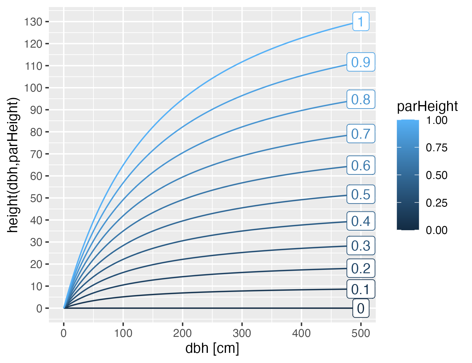
height = \left( \exp \left( \frac{(\text{dbh} \times \text{parHeight})}{(\text{dbh} + 100)} \right) - 1 \right) \times 100 + 0.001

where dbh is the diameter at breast height of the tree in cm and parHeight is an allometric species specific parameter.

All parameters of parHeight from 0 to 1 result in physiologicaly plausible heights. The range from 0.3 to 0.9 results in realistic tree heights. Values of parHeight close to 1 are physiologically almost impossible, below 0.3 is suitable for small tree species and shrubs.

Value

A numeric value representing the calculated height of the tree.

Examples

height(30, 0.5)
height(c(30), c(0.5,0.3))
height(c(30,20), c(0.5))

Index species

Description

Index species

Usage

index_species(pred, species)

Arguments

Value

A torch tensor of pred gathered along its species dimension by species.

Make initial cohorts for FINN

Description

This function prepares obs_df in the exact format expected by FINN::CohortMat$new() and calls it. The required long-table schema is:

• siteID integer index of sites 1..S.

• patchID integer index of patches within site 1..P_s.

• species integer species code 1..sp.

• dbh numeric DBH in cm (either exact or binned midpoints).

• trees integer count of trees in the cohort.

Usage

makeInitCohorts(
  init_trees,
  dbh_binsize = NULL,
  min_dbh = NULL,
  Nspecies,
  treeID_table = FALSE,
  singleCohortTreeNames = NULL
)

Arguments

Details

Aggregates initial trees into cohorts by DBH bins or exact DBH and constructs a FINN::CohortMat object.

Internally calls:

FINN::CohortMat$new(
  obs_df = <data.frame with columns siteID, patchID, species, dbh, trees>,
  dbh    = NULL,
  trees  = NULL,
  species= NULL,
  dims   = c(S, P, K),   # inferred from obs_df
  sp     = Nspecies,     # passed from argument
  device = "cpu"
)

Key fields of the resulting R6 object:

• dbh, trees, species: tensors per cohort.

• dims: integer vector c(S, P, K) for sites, patches, cohorts.

• sp: integer number of species.

• device: "cpu" or "cuda".

• dbh_r, trees_r, species_r: R arrays.

• obsDF2arrays: method converting obs_df into arrays.

Value

If treeID_table = FALSE, a FINN::CohortMat object. If TRUE, a list with:

• initCohort: the CohortMat object.

• init_trees: the obs_df passed to CohortMat$new().

See Also

CohortMat

Create observation data from trees

Description

Derives stand metrics by site/patch/species/year from tree measurements, filters sites, harmonizes years, optionally aggregates by site.

Usage

makeObsData(
  tree_dt,
  plotsize,
  aggregate_by_site = TRUE,
  minNyears = 2,
  fix_period_length = NULL,
  dbh_growth_thresh = c(-10, 50),
  Npatches = NULL,
  Nspecies = NULL,
  NspeciesQuantile = NULL
)

Arguments

Value

A list with:

• obs_dt: observations at site or patch level. growth is the mean relative diameter increment (dbh/dbh_before - 1), and growth_n is how many trees that mean rests on. Both matter: means are aggregated across patches TREE-WEIGHTED (by growth_n), because that is the quantity the model predicts - it simulates sum(g*trees)/sum(trees) over the whole site, so an unweighted mean of patch means would be a different number. growth_n also travels with the response so fit can weight the likelihood by it: 34% of patch-level growth observations rest on a single tree while others average 30+, and the variance of a mean is \sigma^2/n. Mortality comes back as a closed-cohort pair of counts, n_at_risk (trees alive at the start of the interval) and n_died (how many of them were dead at the end), plus the derived rate mort = n_died / n_at_risk (NA where no cohort was at risk). The counts are the binomial response; pass them to fit with mortality = "binomial".

• tree_dt: input trees with added growth fields and species recode.

Mortality

Description

Mortality

Usage

mortality(
  dbh,
  species,
  trees,
  parMort,
  pred,
  light,
  base_steepness = 5,
  debug = FALSE,
  growth = NULL
)

Arguments

Value

A torch tensor of per-cohort mortality probabilities; or, if debug = TRUE, a list of the intermediate components.

Generate random numbers from a uniform distribution

Description

This function generates random numbers from a uniform distribution with specified low and high values and size similar to np.random.uniform in Python.

Usage

np_runif(low, high, size)

Arguments

Value

array A numeric array of random numbers.

Examples

np_runif(0, 1, c(2, 3))

Convert observation data frame to arrays

Description

Convert observation data frame to arrays

Usage

obsDF2arrays(obs_dt, additional_cols = character(0))

Arguments

Value

A list of arrays for species, dbh, trees, and additional columns.

Examples

obs_dt <- data.frame(
  siteID = c(1, 1, 2), patchID = c(1, 2, 1), cohortID = c(1, 1, 2),
  species = c(1, 2, 1), dbh = c(10, 20, 30), trees = c(100, 200, 150),
  height = c(5, 10, 15))
result <- obsDF2arrays(obs_dt, additional_cols = c("height"))

Plot ALE curves of a FINN model

Description

Plots the accumulated local effect (ALE) curves produced by ALE() as a grid: one row per demographic process (growth, mortality, regeneration) and one column per environmental predictor. When several species are present, their curves are overlaid in the same panel as one coloured line each.

Usage

## S3 method for class 'FINNale'
plot(x, process = NULL, scale = FALSE, ...)

Arguments

Value

invisibly, the ggplot object.

Convert Prediction Arrays to Data Frames

Description

This function takes prediction arrays from a model output and converts them into data frames. The data frames can be returned in either 'wide' or 'long' format. The function processes site-level, patch-level, and cohort-level predictions.

Usage

pred2DF(pred, format = "wide")

Arguments

Details

The pred argument should be a list containing at least a Predictions element, which itself is a list of arrays. The arrays represent predictions for different metrics such as dbh/ba, tree counts, AL (aboveground live biomass), growth rates, mortality rates, and regeneration rates for sites, patches, or cohorts. The dimensionality of the arrays should correspond to different factors, such as siteID, year, species, and optionally patch or cohortID.

The function first converts each prediction array into a data frame, properly naming and converting the relevant dimensions. It then merges these data frames by common identifiers such as siteID, year, species, patch, and cohortID. Depending on the format parameter, the data frames are returned in either a wide format (one row per site/patch/cohort per year with multiple columns for different metrics) or a long format (one row per site/patch/cohort per year per metric).

Value

A list of data frames. The list may contain up to three elements: site, patch, and cohort, corresponding to the processed site-level, patch-level, and cohort-level predictions, respectively.

Examples

# a minimal prediction object of the shape pred2DF() expects
# (normally produced by predict()/simulateForest()):
metrics <- c("dbh", "ba", "trees", "growth", "mort", "reg", "r_mean_ha")
arr <- array(1, dim = c(1, 2, 3), dimnames = list(1, 1:2, 1:3))  # [site, year, species]
pred <- list(Predictions = list(Site = stats::setNames(
  lapply(metrics, function(m) arr), metrics)))
result <- pred2DF(pred, format = "long")
head(result$site)

Predict from a FINN model

Description

Predict from a FINN model

Usage

## S3 method for class 'finn_class'
predict(
  object,
  env,
  disturbance = NULL,
  patches = 100L,
  patch_size = 0.1,
  init_cohort = NULL,
  device = c("cpu", "gpu"),
  return_cohorts = FALSE,
  debug = FALSE,
  ...
)

Arguments

Details

Simulate from a (fitted) FINN model. This is an S3 method for the stats::predict generic, so it is dispatched as predict(model, ...).

Value

A named list of predictions. ⁠$long$site⁠ (and ⁠$wide$site⁠) give the site-level results (columns siteID, year, species, variable, value). When return_cohorts is set, ⁠$long$cohort⁠ / ⁠$wide$cohort⁠ add the per-cohort state (dbh, trees, species, growth g, mortality m, ...) for the requested timesteps.

Calculate the regeneration of forest patches based on the input parameters

Description

This function calculates the regeneration of forest patches based on species information, regeneration parameters, prediction values, and available light.

Usage

regeneration(species, parReg, pred, light, debug = FALSE)

Arguments

Value

torch.Tensor Regeneration values for forest patches.

Resolve site, patch, and year indices for FINN inputs

Description

Joins tree, environment, and observation tables; assigns integer indices for site, patch, period; standardizes species coding; and returns aligned data plus optional initial cohorts.

Usage

resolveSiteIDs(tree_dt, env_dt, obs_dt, createInitCohorts = TRUE)

Arguments

Value

A list with:

• siteID_dt: site/patch/year index map.

• tree_dt: tree table with indices and standardized species.

• env_dt: environment table with indices.

• obs_dt: site-aggregated observations by species.

• obs_dt_patches: patch-level observations by species.

• species_dt: species lookup (species, species_name).

• initCohorts (optional): FINN CohortMat object.

• initCohort_dt (optional): trees used to build cohorts.

Generate Cohorts Using Weibull Distribution

Description

This function generates cohort data for tree populations using the Weibull distribution based on specified tree counts, diameter at breast height (DBH) shape, and scale parameters.

Usage

rweibull_cohorts(
  trees = NULL,
  dbh_shape = NULL,
  dbh_scale = NULL,
  dbh_class_range = 1,
  siteID = 1,
  patchID = 1,
  species = 1
)

Arguments

Details

The function generates cohort data by drawing samples from the Weibull distribution for each cohort based on the specified shape and scale parameters. The resulting DBH values are binned into classes, and the cohort data is generated accordingly.

Value

A data frame containing the cohort data with columns for site ID, patch ID, cohort ID, species, number of trees, and DBH.

Examples

obs_df <- rweibull_cohorts(
  trees = c(300, 10),
  dbh_shape = c(3, 3),
  dbh_scale = c(1, 50),
  dbh_class_range = 0.1,
  siteID = c(1, 1),
  patchID = c(1, 1),
  species = c(3, 4)
)
head(obs_df)

Sample poisson relaxed

Description

Sample poisson relaxed

Usage

sample_poisson_relaxed(lmbd, num_samples = 50, temperature = 0.01)

Arguments

Value

A torch tensor of relaxed (differentiable) Poisson samples.

Simulate

Description

Simulate

Usage

simulateForest(
  model,
  env,
  disturbance = NULL,
  patches = 100L,
  patch_size = 0.1,
  init_cohort = NULL,
  device = c("cpu", "gpu"),
  return_cohorts = FALSE,
  debug = FALSE,
  ...
)

Arguments

Details

Simulate from a fitted FINN model. This is a thin, backwards-compatible alias for predict.finn_class; new code should call predict(model, ...) directly.

Value

A named list of simulation results. The patch-averaged, stand-level state variables and demographic rates are in ⁠$long$site⁠ / ⁠$wide$site⁠ (long format: siteID, year, species, variable, value). When return_cohorts is set, ⁠$long$cohort⁠ / ⁠$wide$cohort⁠ hold the raw per-cohort state for the requested timesteps.

Summarise a fitted FINN model

Description

Prints, per process and per species, the environmental variable importance and the average conditional effects. Both are derived from the model's conditional effects, which are computed once and cached — so if ALE() was already run (or a previous summary()), the default path needs no further simulation.

Usage

## S3 method for class 'finn_class'
summary(
  object,
  env = NULL,
  init_cohort = NULL,
  importance = c("ale", "permutation"),
  env_autoscale = TRUE,
  sim_seed = 42L,
  nperm = 20L,
  scale = TRUE,
  ...
)

Arguments

Value

invisibly, a list with importance, average_conditional_effects, and method.